
A residual is how wrong the model predicts each observation. School Stanford University; Course Title ENGLISH 104; Type.
 The center line in I was wondering if someone could tell me what a plot of variable_1 residuals vs variable_2 residuals tell us when each of the two variables were estimated using the same predictors?
 All future courses are included in the purchase of the specialization. When x equals two, we actually have two data points. Close. Plot basics Using ggplot2 package, we will plot the scatterplot of the variable depth vs price as follows Heres the data we will use, one year of marketing spend and company sales by month The graph below is called the Residual vs Chapter 27 Ensemble Methods Chapter 27 Ensemble Methods. One convenient method for testing our model is to compare predicted outcomes to the observed outcomes. Box plots show the distribution of data. Finding predicted outcomes A residual plot is a graph of the datas independent variable values ( x) and the corresponding residual values.
The following code shows how to save the 4 charts for every feature in a separate folder.
P = D B M O V S 100 = 4 7 100 = 57.14. Solution.
Or: you should probably give the output data set a name.
One of the four charts is the residual plot that we can use to detect outliers. The PWRES and NPDEs are computed using the population parameters and the IWRES are computed using the individual parameters. Method 1: Using the plot_regress_exog() plot_regress_exog(): Compare the regression findings to one regressor. Click More.
In researching the easiest way to put these plots together in Python, I stumbled upon the Yellowbrick library.
Then = 0 and e W is a function of the random errors similar to e LS; hence, it follows that a plot of e W versus Y W should generally be a random scatter, similar to the least squares residual plot.. This Article Contains:What Is a Residual Plot and Why Is It Important?Load and Activate the Analysis ToolPakArrange the DataCreate a Residual PlotInterpret the Output Regression Statistics ANOVA Table Coefficients TableA Final Note
In the graph above, you can predict non-zero values for the residuals based on the fitted value. Keeping this in consideration, what is a good residual plot?
See the "Comparing outlier and quantile box plots" section below for another type of box plot.
In the graph above, you can predict non-zero values for the residuals based on the fitted value.
Following Cleveland's examples, the residual-fit spread plot can be used to assess the fit of a regression as follows: Compare the spread of the fit to the spread of the residuals.
The last plot shows very little upwards trend, and the residuals also show no obvious patterns. Adding plots of the residuals vs. the x-value predictors will provide an additional dimension to your analysis that may protect you from making a bad conclusion (an extreme x-value) or from missing a key process effect (variance by a x-value). Apply the formula.
Use the normal probability plot of the residuals to verify the assumption that the residuals are normally distributed.
Cumulating is a kind of smoothing.
Finding Residuals. The sample size for this example is n = 1759.
Pearson residuals scale
Comparing 2 residual scatter plots.
Type of residuals to use in the plot. The residual is 0.5. Homoscedasticity means that the residuals, the difference between the observed value and the predicted value, are equal across all values of your predictor variable.
xn: n + 1 = 0.0005213 0.04102 ( 0.0014479) 0.06236 0.0044554 = 0.0007944. Before this entry discusses the types of individual residual
The fitted values are the ^Y i Y ^ i.
endog vs exog,residuals versus exog, fitted versus exog, and fitted plus residual versus exog are plotted in a 2 by 2 figure.
The course is included in the specialization program, and will be released in . For this example, from the residuals plot we can see the residuals exhibit a good symmetry. Step 1: Compute residuals for each data point. Syntax: statsmodels.graphics.regressionplots.plot_regress_exog(results, exog_idx, fig=None)
(See details for the options available.)
A one-sided formula that specifies a subset of the regressors. We should not use a straight line to model these data.
Step 2: - Draw the residual plot graph. Let me do that in a different color. In such graphs, the residual values are plotted on the y-axis (vertical axis), while the independent variables are plotted on the x-axis (horizontal axis). Construct a residual plot for the data.
Understanding Residuals Plots.
In PASW/SPSS select "Partial residual plots" under the Plots button. Look at the numerical fit results in the Results pane and compare the confidence bounds for the coefficients.
In the Explore Plots menu, under Boxplots click on the button next to Factor levels together if you want to compare the distributions in different groups. I am comparing residuals from model A and model B. Residuals are given by actual (observed) predicted values. It provides, among other things, a nice visualization wrapper around sklearn objects for doing
I have a residuals plot: Definitions: let's call "blue_line" the line that would exist if I were to draw a straight line by fitting to the blue dots (predictions). Because of this, this method is regarded as one of the last resort.
For Anyway, my reply is that these cumulative residual plots dont seem so bad. Residual vs Leverage plot/ Cooks distance plot: The 4th point is the cooks distance plot, which is used to measure the influence of the different plots.
testing for non-proportionality in Cox models.
Answer: Residuals are the differences between the observed values and their corresponding fitted values. In the Options area, select the Plot 2 check box and click Show Plots.The following figure shows the resulting residuals plot.
Suppose that the linear model (39) is correct. I used non-linear random regressions to fit models A and B.
P = D B M O V S 100 = 4 7 100 = 57.14.
The images below compare a scatterplot with its best fit line to the corresponding residual plot: This diagnostic tool tells you what the spread of residuals is like. The residuals versus order plot displays the residuals in the order that the data were collected. Consider the following diagram .
Use the residuals versus order plot to verify the assumption that the residuals are independent from one another. This is a plot of the residuals versus the ascending predicted response values. A residual plot lets you see if your data appears homoscedastic.
endog vs exog,residuals versus exog, fitted versus exog, and fitted plus residual versus exog are plotted in a 2 by 2 figure. Hi.
Syntax: statsmodels.graphics.regressionplots.plot_regress_exog(results, exog_idx, fig=None) Residual Plots. If the points in a residual plot are randomly dispersed around the horizontal axis, a linear regression model is appropriate for the data; otherwise, a non-linear model is more appropriate. Search: Scatter Plot Actual Vs Predicted Python.
after first having saved partial residuals by checking "Partial.
Uploaded By bluesky9700123; Pages 150 This preview shows page 142 - 146 out of 150 pages.
Residuals vs Predicted Plot.
The plot should be a random scatter having a consistent top to bottom range of residuals across the predictions on the X1 axis. Below, the residual plots show three typical patterns. This plot compares the residual to the magnitude of the fitted-value.
Comparing the two residual plots, the residuals of the log-transformed data appear to show a less constant variance than the residuals of the original data. A residual plot is a graph that shows the residuals on the vertical axis and the independent variable on the horizontal axis. library(car) residualPlot(mod1, col='blue', col.quad='blue', A residuals vs. leverage plot is a type of diagnostic plot that allows us to identify influential observations in a regression model.
This is commonly done using the regression residuals. However, let's check some diagnostic residual plots for these two models.
To help interpret a borderline residual plot, a lack-of-fit test for assessing the correctness of the functional part of the model can be used.
So for one of them, the residual is zero.
Examine a lag-1 plot of each residual against the previous residual to identify a serial correlation, where observations are not independent, and there is a correlation between an observation and the previous observation.
There are various kinds of graphs available: Line, Bar, Chart, Histogram etc predicted points of Raw data Figure 2 shows the scatter plot regarding the Actual and Predicted values of the MA data under the best model It reveals various useful insights including outliers 5 as the threshold 6: Actual vs Predicted KKHC 150 One component-plus-residual plot is drawn for each regressor.
Here, one plots the fitted values on the x-axis, and the residuals on the y-axis.
Now for the other one, the residual is negative one.
Biased
Recall that the abline () function adds a line to an existing plot; we just have to specify the intercept and slope. Instead, a more advanced technique should be used. In property development circles, the residual method of valuation is an essential valuation tool for any aspiring investor, as it helps r' 'position-dodge .
Since xn = 0.0014479 and xn 1 = 0.0044554, we can easily get a one-step-ahead prediction. The log-transformed based results are more trustworthy than the results based on the original data.
A residual valuation is a very sensitive topic, with slight variations in its different elements such as rent, initial yield, construction costs, finance rate, and building period. Residuals.
Load the carsmall data set and fit a linear regression model of the mileage as a function of model year, weight, and weight squared.
3.
Posted by 2 years ago.
The linear relationship and constant variance assumptions can be diagnosed using a residuals versus fitted-values plot.
Apply the formula.
If youve never used the tool before, heres how you can activate the Analysis ToolPak: 1. Scatter plots of the Pearson residual, deviance residual, MQR, and RQR versus fitted values under the Poisson, NB, ZIP, and ZINB models in the real data application modeling the number of ER visits.
From the plot we can see that the spread of the residuals tends to be higher for higher fitted values, but it doesnt look serious enough that we would need to make any changes to the model.
Step 3: - Check the randomness of the residuals.
Download scientific diagram | Comparisons of linear regression models and residual plots obtained from the two other methods.
c. Using the estimated line of best fit equation, calculate the residuals for the set of data (round to one decimal place).
There are many types of plots of residuals that allow the model accuracy to be evaluated.
Equally spread residuals across the horizontal line indicate the homoscedasticity of residuals. For example, a fitted value of 8 Sketch a scatter plot of the data b. Interpretation.
Histogram of Residuals. #produce residual vs. fitted plot plot(fitted(model), res) #add a horizontal line at 0 abline(0,0) The x-axis displays the fitted values and the y-axis displays the residuals.
Search: Plot Interrupted Time Series Stata. Step 1. Predicted Value. You may also be interested in qq plots, scale location plots, or the residuals vs leverage plot. fits plot and what they suggest about the appropriateness of the simple linear regression model:The residuals "bounce randomly" around the 0 line. This suggests that the assumption that the relationship is linear is reasonable.The residuals roughly form a "horizontal band" around the 0 line. This suggests that the variances of the error terms are equal.No one residual "stands out" from the basic random pattern of residuals. by asom77 Mon, 20 Oct 2008 20:33:19 GMT . You could use the R option in the MODEL statement.
Search: Plot Glm In R. For example, the data used above could have been input and run as: For example, the data used above could have been input and run as: It's data structure and working environment are perfect for analysis of large sized data ## id model statistic ## 1 Fold01 glm 0 Instead of lm() we use glm() Profile plots (interaction plots) are useful for comparing marginal
load carsmall tbl = table (MPG,Weight); tbl.Year = categorical (Model_Year); mdl = fitlm (tbl, 'MPG ~ Year + Weight^2' );. Plot a histogram of the residuals of a fitted linear regression model. This is the main idea.
Residual plots. The ideal residual plot (called the null residual plot) shows a random scatter of points forming an approximately constant width band around the identity
This part only matters if you have selected multiple variables for the Dependent List. In other words, residual plots attempt to show relationships between the residuals and either the explanatory variables (X 1, X 2, , X p), the fitted values ( i) index numbers (1, 2, , n), or the normal scores (values from a random sample from the standard normal distribution), among others, often using scatterplots. If the residuals are small, the model is good.
If you're seeing this message, it means we're having trouble loading external resources on our website.
First, I'll do this one.
When statisticians want to assess the fit of the model, they often use residual plots. There is some curvature in the scatterplot, which is more obvious in the residual plot.
Predict outcomes and find residuals using matrix operations; Plot residuals on a scatter plot; Add a zero line to your residual plot; Finding residuals.
As percentage is over 33% thus there is difference between Set A and Set B.
is to plot against all numeric regressors.
Residual Plots.
Residual plots are often considered for graphical representation of the residual values.
Quantiles of residual MAI at different stages of StOMP are The residuals are calculated as the difference between the expected value & actual value of the dependent variable.
Now lets look at a problematic residual plot. If you're behind a web filter, please make sure that the domains *.kastatic.org and *.kasandbox.org are unblocked.
(a,c) are the linear Partial residual methods are the most common and preferred methods for. In this post we describe the fitted vs residuals plot, which allows us to detect several types of violations in the linear regression assumptions. When a regression line (or curve) fits the data well, the residual plot has a relatively equal amount of points above and below the x -axis.
The following patterns violate the assumption that the residuals are normally distributed. Populating the interactive namespace from numpy and matplotlib Note: The funnel shape of the dataset showing Heteroscedasticity.
Looking at the residuals distribution on the right-hand side, you can see that the median residuals are the lowest for these two models, with the GLM seeing a higher number of tail residuals. There can be two types of residual plots- linear and nonlinear. Re: Standardized residuals.
It is a visual check for the assumption of constant variance. When comparing your residual plots you will need to incorporate a slide with.
O V S = 13 6 = 7 D B M = 10 3 = 4.
To do this, we'll use the plot.lm command, which is capable of producing six different types of diagnostic plots.
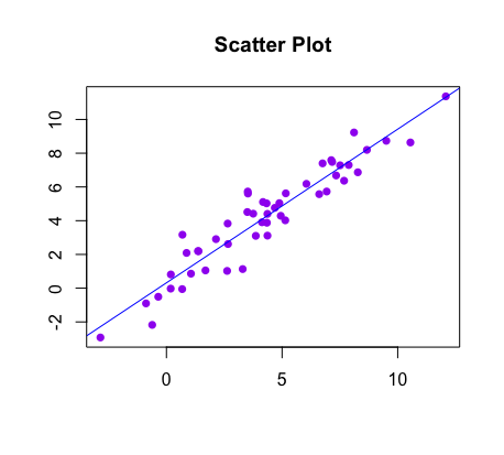
Perhaps the most natural one is simply to plot the fitted line over the scatterplot of the two variables. The second data set shows a pattern in the residuals. The residual plot is a representation of how close each data point is vertically from the graph of the prediction equation from the model. It even shows if the data point is above or below the graph of the prediction equation of the model that is supposed to be best fit for the data.
Residual Plots. The normal probability plot is a graphical tool for comparing a data set with the normal distribution. Click the File tab. A number of different kinds of residuals are used in the analysis of generalized linear models. Independent residuals show no The default ~. 2. Download scientific diagram | QQ plots comparing residual MAI with Gaussian distribution.
Purpose These plots display the PWRES (population weighted residuals), the IWRES (individual weighted residuals), and the NPDEs (normalized prediction distribution errors) as scatter plots with respect to the time or the prediction.
Plots chosen to include in the panel of plots. The position of each dot on the horizontal and vertical axis indicates values for an individual data point. Our first step is enabling the Analysis ToolPak, a built-in data analysis tool that allows you to take a deeper dive into your data. Method 1: Using the plot_regress_exog() plot_regress_exog(): Compare the regression findings to one regressor.
This plot is used for checking the homoscedasticity of residuals. 6.1 Residuals versus Fitted-values Plot: Checks Assumptions #1 and #3. The Cooks distance statistic for every observation Here residual plot exibits a random pattern - First residual is positive, following two are negative, the fourth one is positive, and the last residual is negative. The residual plot shows disagreement between the data and the fitted model. It is likely that Set B is greater than Set A.
The bottom plot displays the residuals relative to the fit, which is the zero line. Draw a Q-Q plot on the right side of the figure, comparing the quantiles of the residuals against quantiles of a standard normal distribution.
The rainbow colors correspond to the distinct values of the response variables ranging from red for the smallest value to blue for the largest value When comparing your residual plots you will need to.
Step 1: Enter the DataEnter the Data First, we will enter the data values. Press Stat, then press EDIT. Perform Linear Regression Next, we will fit a linear regression model to the dataset. Press Stat, then scroll over to CALC. Create the Residual Plot The top plot shows that the residuals are calculated as the vertical distance from the data point to the fitted curve.
For example, the specification terms = ~ . Consider the following diagram . Producing and Interpreting Residuals Plots in In a linear regression analysis it is assumed that the distribution of residuals, (Y Y ) , is, in the population, normal at every level of predicted Y and constant in variance across levels of predicted Y. I shall illustrate how to check that assumption. For example, a fitted value of 8
Also, the points on the residual plot make no distinct pattern. It is likely that Set B is greater than Set A.
Search: Plot Glm In R. The variance of the residuals of a GLM is based on the \(v(\cdot)\) function If you would like to delve deeper into regression diagnostics, two books written by John Fox can help: Applied regression analysis and generalized linear models (2nd ed) and An R and S-Plus companion to applied regression Please click here to find the other part of the Basic GLM Solution. A fit or raw residual is the difference between the observed and predicted values. a. Using two point from the data estimate the equation of the line of best fit. A scatter plot (aka scatter chart, scatter graph) uses dots to represent values for two different numeric variables. Homework Help. 3. Ive used binned residual plots, and I could see how cumulative plots could work too, especially in an area such as highway safety where theres a natural dimension for the smoothing/binning/summing.
The default panel includes a residual plot, a normal quantile plot, an index plot, and a histogram of the residuals.
From the graph.
After you have compared the measured and simulated responses for an estimation, as described in Compare Measured and Simulated Responses, examine the residuals.Select Residuals as the Plot Type for Plot 2 in the New Validation pane. Keep in mind that the residuals should not contain any predictive information. There are also several methods that are important to confirm the adequacy of graphical techniques. Note that this time the default chart is a scatter chart (the last chart type selected) and so we are prompted for both X and Y values (unlike the prompt in Figure 3) Interrupted Time Series Analysis (ITSA) with a single group was used to assess the effects of the policy This paper examines the properties of two nonexperimental Check Residual Plots to display the values of the residuals and graph them.
Keep in mind that the residuals should not contain any predictive information.
Scatter plots are used to observe relationships between variables.
The term box plot refers to an outlier box plot; this plot is also called a box-and-whisker plot or a Tukey box plot. A residual plot is a graph that shows the residuals on the vertical axis and the independent variable on the horizontal axis. O V S = 13 6 = 7 D B M = 10 3 = 4.
We can look at the fitted line in several useful ways.
Now lets look at a problematic residual plot.
Residual. Click OK. For this example, your popup should look like the following: Interpreting Excels Regression Analysis Results.
. The standard residual analysis is very important but may not be fully sufficient. Residual plots are far better than numeric measures in revealing biased models. As percentage is over 33% thus there is difference between Set A and Set B.
Diagnostic residual plots Comparing the (red) linear fit with the (green) quadratic fit visually, it does appear that the latter looks slightly better. residuals" in the "Save New Variables" dialog box under the Save. This problem has been solved! It is a graph plotted between the residuals for a particular regression model and the independent variable. Here is how this type of plot appears in the statistical programming language R: Each observation from the dataset is shown as a single point within the plot. type.
0.
The Residual Plot is graph which is used to check whether the assumptions made in a regression analysis are correct.
The normal probability plot of the residuals should approximately follow a straight line. S-curve implies a distribution with long tails. Examine a sequence plot of the residuals against the order to identify any dependency between the residual and time. The residuals are the ri r i. A Practical Example. Residual plots. When we have the point two comma three, the residual there is zero.
train_color color, default: b Observed Value. Load and Activate the Analysis ToolPak.
Residual plot (method comparison) A residual plot shows the difference between the measured values and the predicted values against the true values. Generalized linear models can be characterized by a variance function that is the variance of a distribution as a function of its mean up to a multiplicative constant. Posted 02-27-2020 10:47 AM (1684 views) | In reply to travis945.
Residual Plots.